Analysing tweets from the Virtual Madrid Open

Tweet map

The tweets come with latitude and longitude coordinates for users who allowed their location to be known.

Using leaflet we can plot the location of the tweets to get an idea of where they are coming from. Unfortunately only a very small proportion of tweets come with location information but we will map those anyway. There are other variables in the dataset that provide information about where the tweet comes from such as city, place but it’s not standardised in any way. These data could be used to derive coordinates if you were stubborn enough.

m <- leaflet() %>%
     addTiles() %>%  # Add default OpenStreetMap map tiles
    #addProviderTiles('Stamen.Toner') %>% 
     addMarkers(lat=tw[!is.na(lat),lat], lng=tw[!is.na(lng),lng],
                     popup=tw[!is.na(lng),text]) 
m  

Even with the small proportion of tweets we can get an idea of where the audience for the tournament is. Leaflet provides nice interactivity, you can the map; if you click on the location pins you get the tweet.

Global audience

Tennis is known to be a very interantional sport with fans all around the world. Separately from mapping the tweet locations we can examine which languages are most represented in the tweet set.

ggplot(tw[,.N,lang][N>50], aes(x=lang,y=N)) + geom_bar(stat="Identity") + theme_bw()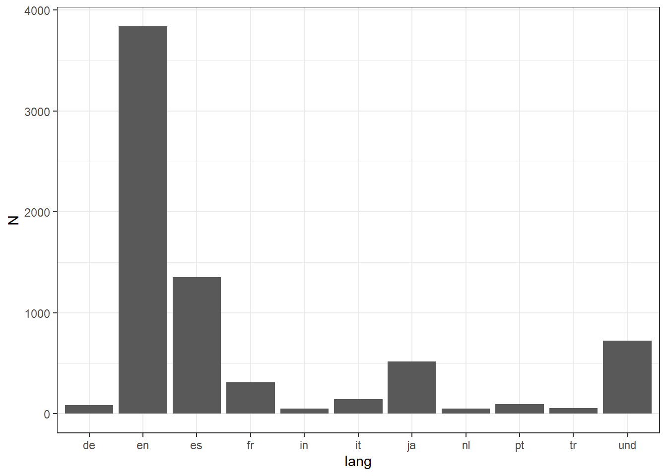

As expected English is the most represented language followed by Spanish. Not a big surprise since the tournament took place in Spain. Japanese comes in a surprising 3rd place due to the presence of Kei Nishikori.

Sentiment analysis

So, how do people feel about this first attempt at an online tournament? We can use sentiment anlysis to go through all the tweets and classify them into positive or negative sentiment. There are several ways to do this, here I will opt for using the sentimentr package which comes with some neat functions that evaluate sentiment directly without having to tokenise or pre-process the data.

Here’s an example of how the package works. We take an example tweet…

exampleText<-tw[lang=="en",text][129]
exampleText

## [1] "I thought the next gen would dominate the virtual #MMOPEN and one of them would be the champs. \n\nIt turned out that one of the big 4 stole the victory.\n\nShame on you, next gen <U+0001F609><U+0001F61D><U+0001F604>"

…and then apply the sentiment_by function to the tweet.

sentiment_by(exampleText)

##    element_id word_count        sd ave_sentiment
## 1:          1         34 0.1980625    -0.1427715

sentiment_by takes the terms in the tweet and associates them to positive or negative sentiments to produce an average sentiment for that tweet. It also outputs thw word count and a standard deviation measure. In this case we can see that the sentiment is negative but given that the stadard deviation is larger than the estimate we cannot be absolutely certain.

Language barrier

Since the sentiment analysis pacakge is geared to work with English only my original idea was to take all the tweets in the most prevalent non-English langauges and translate them to English.

To that end I was planning to use TextBlob; a python pacakge for text analysis that comes with translation capabilities without requiring API keys.

For those paying attention you would have noticed that I casually mention python. That’s right. Using the reticulate package you can import python modules into R! I thought that’s pretty cool and wanted to showcase it in this analysis.

Unfortunately, the translate funtion in TextBlob actually has a limit to how much it can translate and that limit was nowhere close enough to translate all the tweet I have.

In any case, this is how you would go about it:

Import the python module and use it to make a text blob:

require(reticulate)

## Warning: package 'reticulate' was built under R version 3.5.3

tb<-import("textblob") #Import TextBlob
spanishTweet<-tb$TextBlob(tw[lang=="es",][1,text]) #create a blob
spanishTweet

## Hoy debería de dar comienzo el @MutuaMadridOpen. Volveremos a disfrutar como siempre, como nunca. https://t.co/GOT7Yp4Eg8

Do the actual translation:

trans.spanishTweet<-spanishTweet$translate(from_lang = "es", to="en")
trans.spanishTweet

## Today should start @MutuaMadridOpen. We will enjoy again as always, like never before. https://t.co/GOT7Yp4Eg8

The cool thing here is that we are using python within R. This specific case didn’t turn out like I wanted it to but think of the possibilities! Anyway, moving on…

The actual analysis

We are not able to get translated tweet so for now we’ll restrict our view to English tweets only.

Also, I’m interested in the fans’ opinions so I will remove what I call ‘official’ accounts. These include the accounts for the tournament, offcial bodies and broadcasters.

Finally, in my first pass at this I found I was getting some non-tennis related terms back. Turns out the #PlayAtHome term brings in tweets from other events such as concerts, other gaming events, etc. Since this is a quick analysis I decided to get rid of tweets with that hashtag.

We can now calculate sentiment for all the remaining tweets.

twen <- tw[lang=="en"]
offical<-c("MutuaMadridOpen","the_LTA","TennisChannel","WTA","atptour","Tennis","Eurosport_UK")
twen<-twen[!screen_name %in% offical]
twen<-twen[!grep("tHome|thome",text)]
sent <- sentiment_by(get_sentences(twen[,(text)]))

How is the sentiment distributed?

ggplot(sent,aes(ave_sentiment)) + geom_histogram(bins=50) + theme_bw()

There is a big peak at 0 which represents neutral tweets. The distributions to either side of 0 show that sentiment is more positive than negative. So it seems that in general people liked the idea of the virtual Madrid Open.

Let’s remove the neutral-sentiment tweets and plot the histogram again this time looking at the evolution per day.

twen<-bind_cols(twen,sent)
twen[,sent_dir:=ifelse(ave_sentiment<0,"Negative",ifelse(ave_sentiment>0,"Positive","Neutral"))]
ggplot(twen[abs(ave_sentiment)>0 & date(created_at)<"2020-05-01"],aes(ave_sentiment, fill=sent_dir)) + geom_histogram(bins = 50) + facet_wrap(.~date(created_at)) + theme_bw()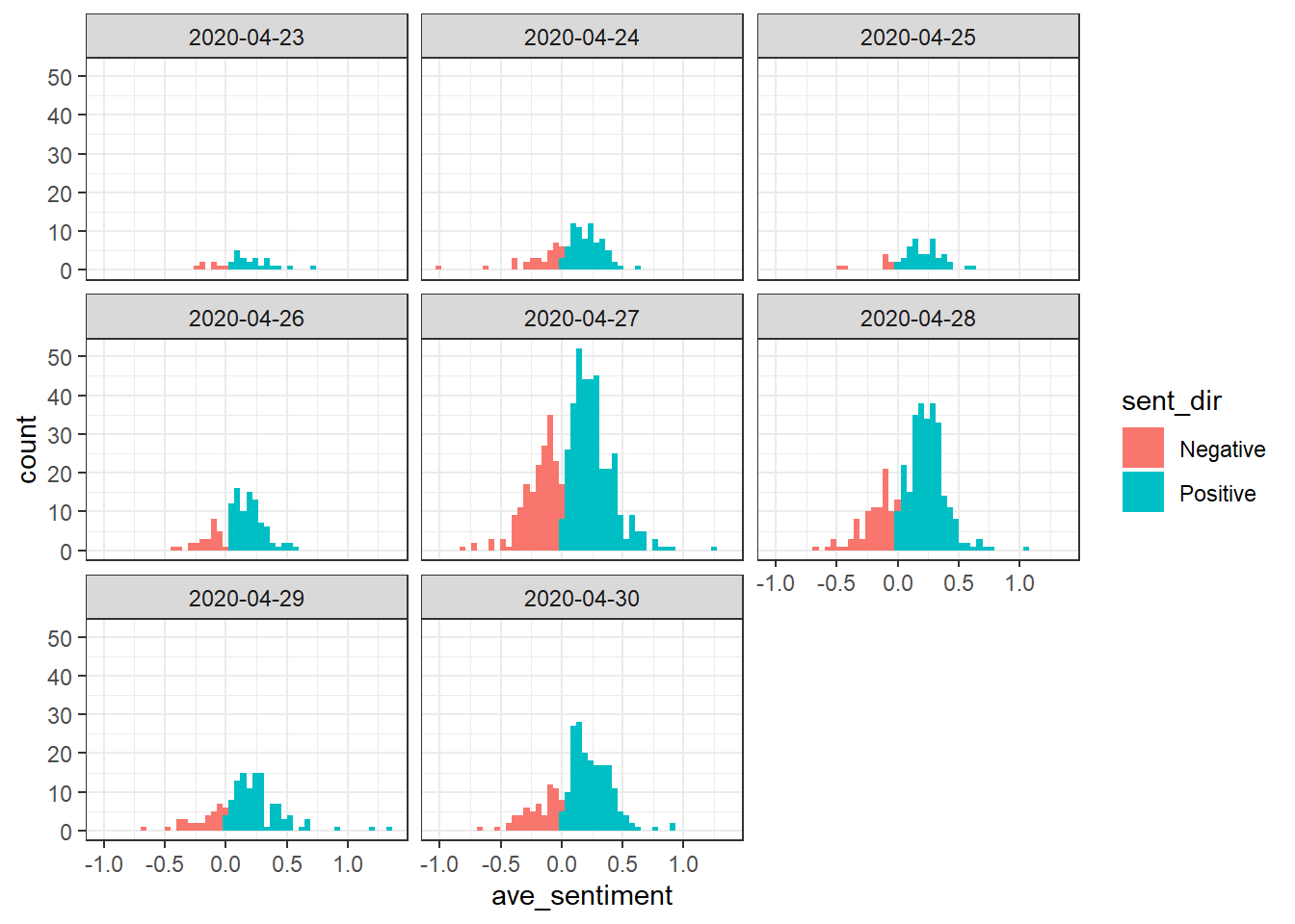

The tournament started on the 27th. From these charts we can see how interest starts building up in the days prior and then peaks on the day the tournament starts. The number of tweets then decreases each day before having a bump on the final day.

In terms of sentiment we can see that positive outweights negative every day but from the histograms it is not easy to see if the proportion changes.

We can tabulate the proportion of postive and negative tweets.

percs<-twen[abs(ave_sentiment)>0 & date(created_at)<"2020-05-01",.N,.(date(created_at),sent_dir)][sent_dir!="Neutral"][,.(sent_dir,p=round(100*N/sum(N))),date]
kable(dcast(percs,sent_dir~date,value.var="p"),format = 'html') %>% kable_styling(bootstrap_options = 'striped')

sent_dir	2020-04-23	2020-04-24	2020-04-25	2020-04-26	2020-04-27	2020-04-28	2020-04-29	2020-04-30
Negative	23	28	15	23	33	24	23	24
Positive	77	72	85	77	67	76	77	76

The proportion of positive sentiment is in the high 70s and 80s for most days. The glaring exception happened on the 27th when the tournament started. Negative sentiment goes up to 32%. Let’s try to figure out why by looking at some wordclouds.

Wordclouds from sentiment terms

The extract_sentiment_terms function tells us which terms in the tweets contributed to the sentiment score.

terms<-extract_sentiment_terms((twen[,text]))

We can visualise these terms using the wordcloud package. I will make one cloud for positive terms and one for negative ones.

Before constructing the clouds I’m removing stop words, common terms like ‘at’,‘the’,‘in’, that do not contribute to sentiment. Apart from the terms in the stop_words array provided by the tidytext pacakge I’m also removing some custom terms that will be very common in our tweet set but which won’t tell us much about sentiment.

The postive-term cloud:

my_sw<-c(stop_words$word,"virtual","pro","play","game","tennis","players","madrid","match","video","games","player","players","tournament")

u<-data.table(words=unlist(terms[,positive]))[,.N,words][order(-N)]
u<-u[!words %in% my_sw]
par(mfrow=c(1,2))
wc_pos<-wordcloud(words = u$words, freq = u$N, min.freq = 1,max.words=200, random.order=FALSE, rot.per=0.35,colors=brewer.pal(8, "Dark2"))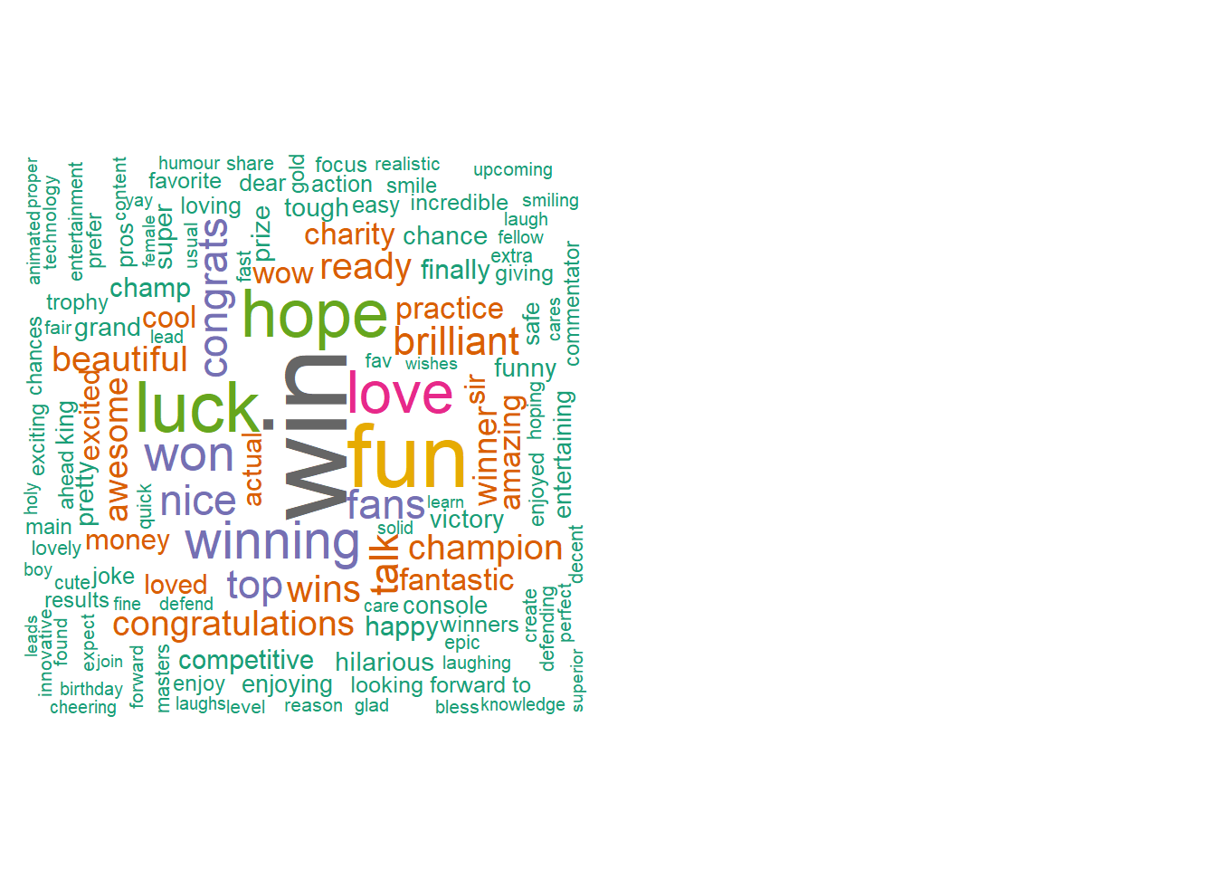

Positive terms are what you would expect with things like “win”, “fun”, “luck” and “congrats” having the biggest size.

The negative-term cloud:

u<-data.table(words=unlist(terms[,negative]))[,.N,words][order(-N)]
u<-u[!words %in% my_sw]
wc_neg<-wordcloud(words = u$words, freq = u$N, min.freq = 1,max.words=200, random.order=FALSE, rot.per=0.35,colors=brewer.pal(8, "Dark2"))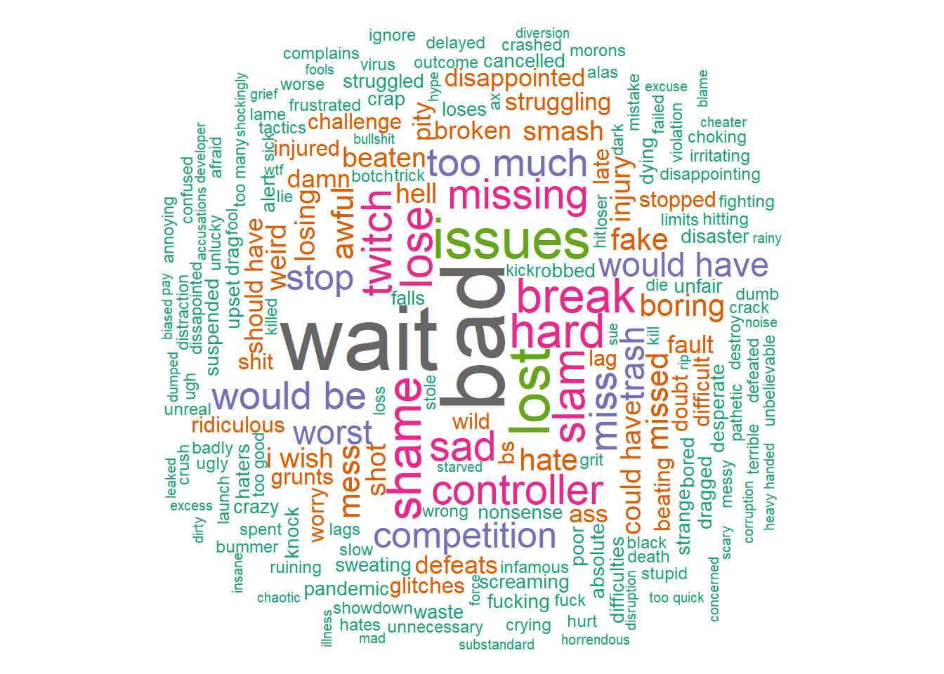

Regarding negative terms apart from traditionally negative words it is interesting to see things like “issues”, “twitch”, “controller”. “Twitch” could be fans aluding to the fact that it would have been better to hold the tournament in that platform.

Wordclouds from tweets

Finally, we can also build wordlcouds directly from the tweets. We can make a positive-term wordcloud from the tweets with positive average sentiment and analogously for the negative terms.

First, let’s do a quick cleaning of the text data so it doesn’t appear in the clouds.

twen[,text2 := gsub("https\\S*", "", text)]
twen[,text2 := gsub("@\\S*", "", text2) ]
twen[,text2 := gsub("#\\S*", "", text2) ]
twen[,text2 := gsub("amp", "", text2) ]
twen[,text2 := gsub("[\r\n]", "", text2)]
twen[,text2 := gsub("[[:punct:]]", "", text2)]

We now make the wordclouds.

u<-unnest_tokens(twen[!grep("atHome",text)][ave_sentiment>0,.(text2)],words,text2)[,.N,words][order(-N)]
u<-u[!words %in% my_sw]
wordcloud(words = u$words, freq = u$N, min.freq = 5,max.words=200, random.order=FALSE, rot.per=0.35,colors=brewer.pal(8, "Dark2"),scale = c(1.5,0.5))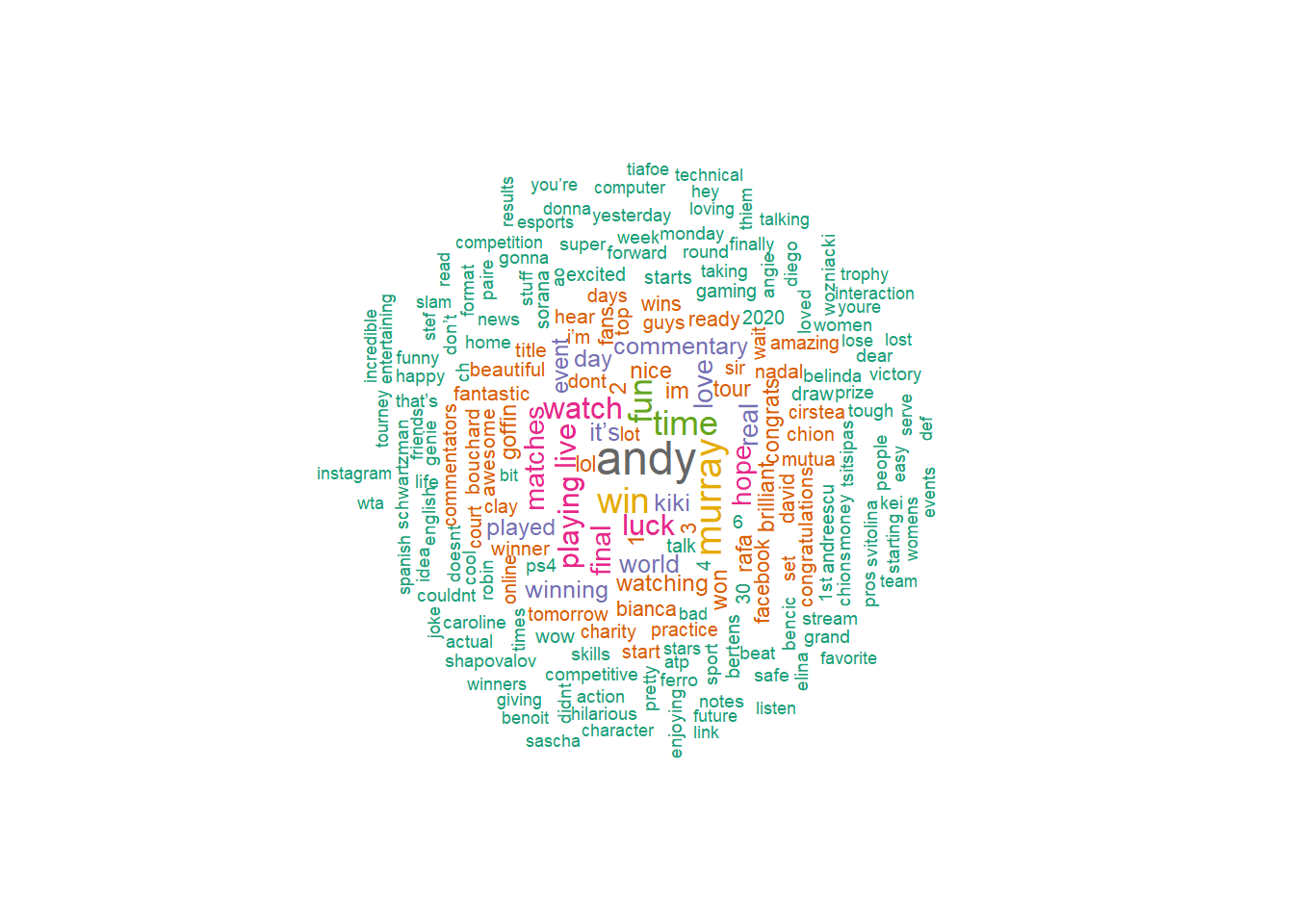

This time there’s a lot more terms in the wordcloud because the tweets are richer than the extracted term data. Many of the extra terms are realted to player names. Otherwise we see similar type of words as in the extracted term cloud.

u<-unnest_tokens(twen[!grep("atHome",text)][ave_sentiment<0,.(text2)],words,text2)[,.N,words][order(-N)]
u<-u[!words %in% my_sw]
wordcloud(words = u$words, freq = u$N, min.freq = 3,max.words=200, random.order=FALSE, rot.per=0.35,colors=brewer.pal(8, "Dark2"), scale = c(1.5,0.5))

The negative-tweet word cloud also now includes a lot of player names but we can see more hints of what poeple didn’t like so much, i.e., terms like “commentators”," internet“,”wait" and “facebook”.

Conclusion

We went on a whirlwind tour of several packages that can be used to analyse tweets or other types of text data. This is really only scratching the surface of what can be done so it will be interesting to keep exploring these packages and other ones such as spacy and quanteda which are used to do more complex things like parts-of-speech tagging, more comprehensive feature extraction and they also support more language models.

In terms of the tournament, there were some teething issues like the choice of streaming platform, players with bad internet connections and too much commentary rather than having players mic’ed up. However, the overall sentiment was positive and people seemed to welcome this type of innovation from the organisers. We’ll see how future online tournaments fare.